Quantopian How to Use Custom Uploaded Data

Last Updated on January eleven, 2021
If y'all desire to backtest a trading strategy using Python, you lot tin can 1) run your backtests with pre-existing libraries, 2) build your own backtester, or 3) utilise a cloud trading platform.
Option one is our selection. It gets the chore done fast and everything is safely stored on your local figurer.
(After y'all become an algorithmic trading good, you can consider option 2 if the current available solutions don't fulfill your needs.)
There are ii pop libraries for backtesting. Backtrader is 1 of them. The other is Zipline.
In this commodity, we will focus on Backtrader.
Tabular array of Contents
- What is Backtrader?
- Why should I learn Backtrader?
- Why shouldn't I learn backtrader?
- Overview of how Backtrader works
- How to install Backtrader
- Choosing which IDE to utilize with Backtrader
- How to configure the bones Backtrader setup
- How to get data and import it into Backtrader
- How to print or log data using the strategy class in Backtrader
- How to run a backtest using Backtrader
- How to utilize the built-in crossover indicator
- How to run optimization in Backtrader
- How to build a stock screener in Backtrader
- How to lawmaking an indicator in Backtrader
- How to plot in Backtrader
- How to utilize alternative data in Backtrader
- How to add together visual stats to a backtest
- How to salvage backtest information to a CSV file
- Alternatives to Backtrader
- Terminal Thoughts on Backtrader
- Download all code and data
What is Backtrader?
Backtrader is a Python library that aids in strategy development and testing for traders of the financial markets.
Information technology is an open-source framework that allows for strategy testing on historical data. Further, it can be used to optimize strategies, create visual plots, and can even be used for live trading.
Why should I learn Backtrader?
Using Backtrader tin can save you lot endless hours of writing lawmaking to test out market strategies.
With a large customs, and an active forum, you can easily notice assistance with any problems holding upward your development. Further, the extensive documentation on Backtrader'southward website might even atomic number 82 to the discovery of a crucial component for your strategy.
Here are some of the things Backtrader excels at:
Backtesting – This might seem like an obvious one but Backtrader removes the tedious procedure of cleaning upward your data and iterating through it to test strategies. It has congenital-in templates to apply for various data sources to make importing data easier.
Optimizing – Adjusting a few parameters tin can sometimes be the difference between a assisting strategy and an unprofitable i. Later running a backtest, optimizing is easily done past changing a few lines of code.
Plotting – If you've worked with a few Python plotting libraries, you'll know these are not always easy to configure, peculiarly the first fourth dimension effectually. A complex chart tin can exist created with a single line of code.
Indicators – Most of the popular indicators are already programmed in the Backtrader platform. This is specially useful if you want to test out an indicator but you're non sure how constructive information technology volition exist. Rather than trying to figure out the math behind the indicator, and how to code it, yous tin test it out first in Backtrader, probably with ane line of code.
Back up for Complex Strategies – Desire to take a signal from one dataset and execute a trade on another? Does your strategy involve multiple timeframes? Or do you demand to resample data? Backtrader has accounted for the diverse ways traders approach the markets and has extensive back up.
Open up Source – There is a lot of benefit to using open-source software, here are a few of them:
- You lot have full admission to all the individual components and can build on them if desired.
- There's no need to upload your strategy to a third-political party server which eases concerns over confidentiality.
- You're non obligated to upgrade and bargain with unwanted changes as you might with software from a corporation. A expert instance of this is when Quantopian discontinued live trading a few years ago. It forced many users to drift to a different platform which tin can be cumbersome.
Active Development – This might be one area where Backtrader specially stands out. The framework was originally adult in 2015 and constant improvements have been made since then. Just a few weeks ago, a pandas-based technical assay library was released to address bug in the popular and commonly used TA-Lib framework. Farther, with a wide user base, there is also agile third-party evolution.
Live Trading – If you lot're happy with your backtesting results, it is like shooting fish in a barrel to migrate to a live environs within Backtrader. This is especially useful if you lot plan to employ the built-in indicators offered by the platform.
» Backtrader is used for backtesting and not live trading.
QuantConnect is a browser-based platform that allows both backtesting and alive trading.
Link: QuantConnect – A Complete Guide
Content Highlights:
- Create strategies based on alpha factors such as sentiment, crypto, corporate actions and macro data (information provided past QuantConnect).
- Backtest and trade a wide array of asset classes and industries ETFs (data provided past QuantConnect).
- License strategies to hedge fund (while you go along the IP) via QuantConnect's Alpha Stream.
Why shouldn't I learn Backtrader?
A potentially steep learning curve – At that place is a lot you can do with Backtrader, it is very comprehensive. Simply the boosted functionality can be seen as a double-edged sword. It will have some time to empathize the syntax and logic that are used.
Understanding the Library – Building on the previous point, it is a practiced idea to look through the source code of any library to go a amend understanding of the framework. When decompressing the source code, 470 items were extracted. Granted, some of these are examples or datasets. There were also several scripts no longer in use. Nevertheless, there is a lot to go through.
Having to supply data – At 1 bespeak, integration with the Yahoo Finance API took intendance of this issue. The API has since deprecated and you lot will at present need to source and supply data. In that location are methods to connect with a banker that can address this result, admitting not all that straight forward.
Creating your own framework – Some people prefer to have a full agreement of their software and would rather create a backtesting platform by themselves. In most cases, this will exist a lot more work, just in that location are obvious benefits. If you lot're looking to just get a general thought well-nigh a simple strategy, information technology might be easier to just try and iterate over historical information versus learning the library.
Overview of how Backtrader works
Backtrader shows you how your strategy might perform in the market by testing it against past price data.
The library'south about basic functionality is to iterate through historical data and to simulate the execution of trades based on signals given by your strategy.
It extends on this functionality in many ways. A Backtrader "analyzer" tin be added to provide useful statistics. We volition show an example of this using the commonly used Sharpe Ratio in a optimization examination later in this tutorial.
On the field of study of optimization, it'southward clear a lot of thought has been put in to speeding upward the testing of strategies with different parameters. The built in optimization module uses multiprocessing, fully utilizing your multiple CPU cores to speed upwardly the procedure.
Lastly, Backtrader utilizes the well-known matplotlib library to create charts at the cease of your backtest, if desired.
How to install Backtrader
The easiest way to install Backtrader is by command line. Simply blazon in pip install backtrader.
If you plan to employ the charting functionality, you should take matplotlib installed. The minimum version requirement for matplotlib is ane.4.one.
You can confirm it is installed on your arrangement by typing in pip listing from the control line to show installed Python packages.
If yous need to install it, you tin can do so either via pip install backtrader[plotting] or pip install matplotlib.
Alternatively, you can run Backtrader from source. Download the zero file from the Backtrader GitHub page – https://github.com/mementum/backtrader/annal/master.nil and unzip the backtrader directory inside your project file.
Choosing which IDE to use with Backtrader
Before diving into lawmaking, let'southward have a cursory moment to discuss IDE'south.
An IDE, or Integrated Development Environment, is simply an editor to write and debug your code from. There are several popular IDE'due south out there and choosing the right i often comes downwardly to personal preference.
Python comes bundled with an IDE called IDLE. Some of the popular 3rd-political party Python IDE's out in that location include VS Code, Sublime Text, PyCharm and Spyder.
Some other consideration is whether to employ an interactive IDE or not. A popular choice when it comes to interactive IDE's is Jupyter Notebook.
Interactive IDE's take the boosted capability of executing selected blocks of lawmaking without running your entire script. This is very useful when testing out a new library as you can try out unlike functions without having to comment out or delete your previous lawmaking block.
While it is possible to use interactive IDE's for some functionality in Backtrader, it is not recommended. There are sure functions, such as optimization, that require multiprocessing which does non piece of work well with interactive IDE's.
If yous decide to use an interactive IDE, yous should exist able to follow along until the optimization portion of this tutorial. Only make certain to point to the exact path where your CSV data file is stored on the next part which covers adding data.
How to configure the bones Backtrader setup
There are two main components to setting up your basic Backtrader script. The strategy class, and the cerebro engine.
import backtrader as bt form MyStrategy(bt.Strategy): def side by side(self): laissez passer #Do something #Instantiate Cerebro engine cerebro = bt.Cerebro() #Add strategy to Cerebro cerebro.addstrategy(MyStrategy) #Run Cerebro Engine cerebro.run() We will go into the strategy class in more detail in the examples that follow. This is where all the logic goes in determining and executing your trade signals. Information technology is likewise where indicators can be created or called, and where you can determine what get's logged or printed to screen.
The cerebro engine is the core of Backtrader. This is the master class and we will add our data and strategies to it before somewhen calling the cerebro.run() command.
How to get information and import it into Backtrader
There are several means to get data. If you're already signed upwards with a banker, you might have API admission to catch historical data.
Alternatively, at that place are many third-party API'southward available that allow you to download historical information from within your Python console.
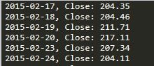
For our case, we will download data in CSV format directly from the Yahoo Finance website.
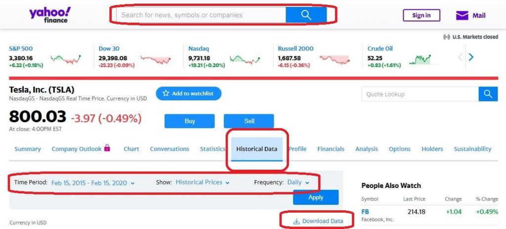
Just navigate to the Yahoo Finance website and enter in the ticker or company name for the data you're looking for. Then, click on the Historical Data tab, select your Time Flow, and click on Apply. At that place will be a Download Information link which volition save the CSV file to your hard drive.
It'due south a practiced idea to copy the CSV file over to your projection directory. Otherwise, you lot will have to specify a total pathname when calculation your data to cerebro.
We can add our data to Backtrader by using the congenital-in feeds template specifically for Yahoo Finance. The template will take care of any formatting required for Backtrader to properly read the data.
information = bt.feeds.YahooFinanceCSVData(dataname='TSLA.csv') cerebro.adddata(data)
In the above example, nosotros've assigned the CSV dataset to a variable named data. The adjacent step is to add this to cerebro.
Calculation data can be done at whatsoever point betwixt instantiating cerebro and calling the cerebro.run() command. There are several additional parameters we can specify when loading our data. We volition explore this farther in our adjacent instance.
How to print or log data using the strategy class in Backtrader
To go a fleck more familiar with the Strategy class in Backtrader, we will create a simple script that prints the endmost prices for our dataset. The Strategy class is where we will be spending virtually of our time within Backtrader.
The first matter we will do is create a new class called PrintClose which inherits the Backtrader Strategy class.
import backtrader as bt class PrintClose(bt.Strategy): def __init__(cocky): #Continue a reference to the "close" line in the data[0] dataseries self.dataclose = cocky.datas[0].shut In the __init__ role in a higher place, we've created a variable called dataclose to make information technology easier to refer to the closing cost afterward on. You will notice that the closing price is stored in datas[0].close. We tin simply as easily access the open price by referencing datas[0].open. If you're using multiple information feeds, you can access your second feed past referencing datas[ane].close, merely more on that later.
An of import feature of Backtrader is accessing historical data which we tin now practise via the dataclose variable. Every bit Backtrader iterates through historical data, this variable will get updated with the latest price from dataclose[0]. We tin can also look dorsum to the prior information points by accessing the negative alphabetize of dataclose. Hither is an example.
if dataclose[0] > dataclose [-1]: pass # practice something
The above code checks to see if the almost recent close is larger than the prior close. We can but equally easily access the second terminal closing price by changing the index like this: dataclose[-ii]
The next pace is to create a logging function.
def log(cocky, txt, dt=None): dt = dt or self.datas[0].datetime.appointment(0) print(f'{dt.isoformat()} {txt}') #Print engagement and shut The log function allows united states of america to pass in data via the txt variable that we desire to output to the screen. It will try to catch datetime values from the nigh contempo data point,if available, and log it to the screen.
Now that our printing/logging part has been defined, nosotros will overwrite the adjacent function. This is the virtually of import part of the strategy class as most of our code will get executed here. This part gets chosen every fourth dimension Backtrader iterates over the side by side new data bespeak.
def adjacent(self): self.log('Close: ', cocky.dataclose[0]) All we volition do for now is log the closing price.
This is what our complete script looks similar at this point:
import backtrader every bit bt course PrintClose(bt.Strategy): def __init__(cocky): #Continue a reference to the "close" line in the data[0] dataseries cocky.dataclose = self.datas[0].close def log(self, txt, dt=None): dt = dt or self.datas[0].datetime.engagement(0) print(f'{dt.isoformat()} {txt}') #Print date and close def next(self): self.log('Shut: ', cocky.dataclose[0]) #Instantiate Cerebro engine cerebro = bt.Cerebro() #Add together information feed to Cerebro data = bt.feeds.YahooFinanceCSVData(dataname='TSLA.csv') cerebro.adddata(data) #Add strategy to Cerebro cerebro.addstrategy(PrintClose) #Run Cerebro Engine cerebro.run() And this is what your output should look like:
From this point on, the structure of our script will mostly remain the same and we will write the bulk of our strategies under the next part of the Strategy grade.
How to run a backtest using Backtrader
We've installed Backtrader, downloaded some historical information, and written our basic script. The next step is to backtest a strategy.
We will test out a moving average crossover strategy. Essentially, information technology involves monitoring ii moving averages and taking a trade when one crosses the other.
The moving average crossover strategy is to trading what the Hello World script is to programming. Neither will likely ever be used in the existent world and are mostly used for illustrative purposes. In other words, we don't expect the strategy to exist a profitable i.
There are a few things we will exercise earlier diving into the strategy. First, we will separate our strategy into its own file. Throughout this tutorial, nosotros will go over several examples and separating out the strategies from the main script volition keep the code in a nice clean format.
The primary script, which volition have everything cerebro related, will only have small changes throughout the tutorial while nigh of the work will be done in the strategies script.
The strategies script will be appropriately named strategies.py.
import backtrader as bt class PrintClose(bt.Strategy): def __init__(self): #Keep a reference to the "close" line in the data[0] dataseries self.dataclose = self.datas[0].close def log(self, txt, dt=None): dt = dt or self.datas[0].datetime.date(0) print(f'{dt.isoformat()} {txt}') #Print date and close def next(cocky): self.log('Close: ', self.dataclose[0]) We also take to carve up our data into two parts. This manner, we can test our strategy on the first role, run some optimization, and and so see how it performs with our optimized parameters on the second set of data.
If you lot've heard the terms in-sample data, or out-of-sample data, this is what information technology is referring to. Out-of-sample data is simply information prepare aside for testing after optimization.
There are a lot of benefits to testing and optimizing this way, take a look at What is a Walk-Frontward Optimization and How to Run It? if you lot'd like to get a more than thorough understanding of the methodology.
To separate the data, we set a from date and to date when loading our data. Don't forget to import the DateTime module for this office.
Here is our updated main script which will be chosen btmain.py:
import datetime import backtrader equally bt from strategies import * # Instantiate Cerebro engine cerebro = bt.Cerebro() # Set data parameters and add to Cerebro data = bt.feeds.YahooFinanceCSVData( dataname='TSLA.csv', fromdate=datetime.datetime(2016, 1, 1), todate=datetime.datetime(2017, 12, 25), ) # settings for out-of-sample data # fromdate=datetime.datetime(2018, 1, 1), # todate=datetime.datetime(2019, 12, 25)) cerebro.adddata(data) # Add together strategy to Cerebro cerebro.addstrategy(AverageTrueRange) # Default position size cerebro.addsizer(bt.sizers.SizerFix, pale=3) if __name__ == '__main__': # Run Cerebro Engine start_portfolio_value = cerebro.broker.getvalue() cerebro.run() end_portfolio_value = cerebro.broker.getvalue() pnl = end_portfolio_value - start_portfolio_value print(f'Starting Portfolio Value: {start_portfolio_value:2f}') impress(f'Final Portfolio Value: {end_portfolio_value:2f}') impress(f'PnL: {pnl:.2f}') Nosotros have included from strategy import * which will get in easier to telephone call new strategies from the master script equally we create them. Likewise included towards the terminate of the script are some details regarding portfolio values and our default position size, which has been ready to iii shares.
The command cerebro.broker.getvalue() allows y'all to obtain the value of the portfolio at any time. We grab the starting value by calling it before running cerebro and so call it in one case again subsequently to get the catastrophe portfolio value. We can see our turn a profit or loss by subtracting the end value from the starting value.
Let's get started on our strategy!
class MAcrossover(bt.Strategy): # Moving average parameters params = (('pfast',20),('pslow',50),) def log(self, txt, dt=None): dt = dt or self.datas[0].datetime.date(0) print(f'{dt.isoformat()} {txt}') # Comment this line when running optimization def __init__(self): self.dataclose = self.datas[0].close # Society variable will contain ongoing order details/condition self.order = None # Instantiate moving averages cocky.slow_sma = bt.indicators.MovingAverageSimple(cocky.datas[0], period=cocky.params.pslow) self.fast_sma = bt.indicators.MovingAverageSimple(cocky.datas[0], period=self.params.pfast) In the code in a higher place, we've created a new form called MAcrossover which inherits from the Backtrader Strategy class.
We've set some parameters for our moving average rather than hard coding them. This volition make it easier to optimize the strategy later on.
There are a few new items under the __init__ function. We've created an order variable which volition store ongoing order details and the order status. This way we will know if we are currently in a trade or if an guild is awaiting.
One thing to note about Backtrader is that when it receives a buy or sell point, we tin instruct it to create an order. All the same, that order won't exist executed until the adjacent bar is called, at whatever price that may be.
We've likewise created ii moving averages by utilizing indicators built into Backtrader. The benefit of using built-in indicators is that Backtrader won't get-go looking for orders until this data is fabricated available.
To clarify, the larger of the two moving averages uses an average of the last 50 closing prices. That means the first 50 data points volition have a NaN moving average value. Backtrader knows not to await for orders until we have valid moving average data.
The next item we will overwrite is the notify_order function. This is where everything related to trade orders gets processed.
def notify_order(self, order): if order.condition in [order.Submitted, order.Accustomed]: # An agile Buy/Sell club has been submitted/accepted - Nothing to practise return # Check if an lodge has been completed # Attention: banker could reject order if not enough cash if order.status in [club.Completed]: if society.isbuy(): self.log(f'Buy EXECUTED, {order.executed.price:.2f}') elif order.issell(): cocky.log(f'SELL EXECUTED, {guild.executed.cost:.2f}') self.bar_executed = len(self) elif order.condition in [order.Canceled, order.Margin, guild.Rejected]: self.log('Guild Canceled/Margin/Rejected') # Reset orders self.order = None What the above lawmaking does is allow us to log when an order gets executed, and at what price. This section will as well provide notification in instance an society didn't become through.
Lastly, we accept the next function which contains all of our merchandise logic.
def next(self): # Cheque for open orders if self.order: return # Bank check if nosotros are in the market if not self.position: # We are not in the market, look for a signal to OPEN trades #If the 20 SMA is to a higher place the fifty SMA if self.fast_sma[0] > self.slow_sma[0] and self.fast_sma[-1] < self.slow_sma[-1]: self.log(f'BUY CREATE {self.dataclose[0]:2f}') # Keep runway of the created social club to avoid a 2nd order self.club = self.buy() #Otherwise if the twenty SMA is below the 50 SMA elif self.fast_sma[0] < cocky.slow_sma[0] and self.fast_sma[-ane] > self.slow_sma[-1]: self.log(f'SELL CREATE {self.dataclose[0]:2f}') # Keep runway of the created order to avoid a 2nd club self.order = cocky.sell() else: # Nosotros are already in the market, wait for a bespeak to Shut trades if len(self) >= (self.bar_executed + 5): cocky.log(f'Shut CREATE {self.dataclose[0]:2f}') cocky.order = self.close() We outset check for an active order in which example we don't desire to do annihilation. For this strategy, nosotros only want to exist in one position at a fourth dimension.
If nosotros're not in the marketplace, we tin can beginning looking for a moving average crossover. 1 affair to be mindful of in this strategy is that our signal comes from the cantankerous of one moving average over another.
To satisfy that requirement, we check to see if the xx moving average was below the 50 moving boilerplate on the last candle simply is in a higher place it on the current candle or vice versa. This confirms a cross has taken identify. Otherwise, we would be constantly getting a betoken.
Finally, nosotros have our else statement which gets executed if we are already in the market. For the exit strategy, nosotros will only exit 5 bars after inbound the merchandise.
On running the code, the script will output all of our trades and print a terminal PnL at the end. In this case, we had a $79 turn a profit.
I affair to keep in heed when testing strategies is that the script tin can end with an open trade in the system. One way to check if in that location are any open trades is to ensure 'CLOSE CREATE' is the 2d last line output before the portfolio values are printed. Otherwise, an open trade will likely skew your PnL results.
How to use the built-in crossover indicator
In our moving average cross over example, we coded the logic involved in determining if the two moving averages were crossing. Backtrader has developed an indicator that tin determine this which can brand things a bit easier.
To employ the built-in indicator, instantiate it in the __init__ role as follows: self.crossover = bt.indicators.CrossOver(self.fast_sma, self.slow_sma)
if cocky.crossover > 0: # Fast ma crosses to a higher place slow ma pass # Indicate for buy club elif cocky.crossover < 0: # Fast ma crosses below slow ma laissez passer # Signal for sell order How to run optimization in Backtrader
Our next step is to try and see if we can increase our profits past irresolute some of the moving average parameters.
In the Strategy, we will comment out the print argument in the log role. Optimizing involves several backtests with diverse parameters and we don't demand to log and go through every trade that takes place.
Instead, we will judge the strategy performance based on the Sharpe Ratio.
At that place are a number of changes to the chief script file to run the optimization. Here is the code for the updated chief script:
import datetime import backtrader as bt from strategies import * cerebro = bt.Cerebro(optreturn=Fake) #Set up data parameters and add to Cerebro data = bt.feeds.YahooFinanceCSVData( dataname='TSLA.csv', fromdate=datetime.datetime(2016, 1, 1), todate=datetime.datetime(2017, 12, 25)) #settings for out-of-sample information #fromdate=datetime.datetime(2018, 1, 1), #todate=datetime.datetime(2019, 12, 25)) cerebro.adddata(data) #Add strategy to Cerebro cerebro.addanalyzer(bt.analyzers.SharpeRatio, _name='sharpe_ratio') cerebro.optstrategy(MAcrossover, pfast=range(5, twenty), pslow=range(l, 100)) #Default position size cerebro.addsizer(bt.sizers.SizerFix, stake=3) if __name__ == '__main__': optimized_runs = cerebro.run() final_results_list = [] for run in optimized_runs: for strategy in run: PnL = circular(strategy.broker.get_value() - 10000,2) sharpe = strategy.analyzers.sharpe_ratio.get_analysis() final_results_list.suspend([strategy.params.pfast, strategy.params.pslow, PnL, sharpe['sharperatio']]) sort_by_sharpe = sorted(final_results_list, key=lambda 10: x[3], reverse=True) for line in sort_by_sharpe[:v]: print(line) Permit's run through some of the major changes. When instantiating cerebro, the optreturn=Imitation parameter was added in. Cerebro removes some data output when running optimization to ameliorate speed. Nevertheless, we require this data, hence the additional parameter.
cerebro.addstrategy was removed and replaced with cerebro.optstrategy. We've likewise added additional parameters that specify a range of values to optimize the moving averages for. Further, an analyzer was added which will calculate the Sharpe Ratio for our results.
You may have noticed that we added an if __name__ == '__main__': block. In our testing, we ran into an fault without information technology in place.
The optimized results are being stored in the variable optimized_runs in the form of a list of lists. The bottom department of the code iterates through the lists to grab the values that we need and appends it to a newly created list.
The last 3 lines of the code sorts the list and prints out the superlative five values. This is what our results looked like:
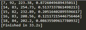
It looks like we accept a clear winner. A flow of 7 for the fast moving boilerplate and a period of 92 for the slow moving average produces a notably higher result for the Sharpe Ratio.
Now information technology'south time to run some backtests on the out-of-sample data. All it takes is a simple change to the data parameters.
fromdate=datetime.datetime(2018, 1, 1), todate=datetime.datetime(2019, 12, 25)) Our backtest shows a loss of $63.42 with the same settings we used in our original test, but on the out-of-sample data. Here is the result afterward irresolute the moving average settings to the optimized parameters.
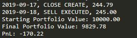
A loss of $170.22, even greater than our original settings although this was expected equally a few things are impacting our figures.
First, the moving average cross over is an unsophisticated strategy that was expected to produce a loss. The only surprise here was that information technology produced a turn a profit in our get-go run.
Second, this is a cracking instance of overfitting. If you lot're not familiar with overfitting, definitely check out What is Overfitting in Trading? – it is a crucial element of strategy development.
How to build a stock screener in Backtrader
Screeners are usually used to filter out stocks based on sure parameters. In that location aren't a lot of easy ways to look back to a certain engagement and see what results a stock screener might take spit out. Fortunately, Backtrader offers exactly this.
We will exam out this functionality past edifice a screener that filters out stocks that are trading two standard deviations beneath the average price over the prior 20 days.
We will starting time by creating a subclass of the Backtrader Analyzer class which will form the 'screener' component of our strategy.
grade Screener_SMA(bt.Analyzer): params = (('catamenia',20), ('devfactor',2),) def start(self): self.bband = {information: bt.indicators.BollingerBands(data, menstruation=cocky.params.period, devfactor=cocky.params.devfactor) for information in self.datas} def stop(cocky): self.rets['over'] = list() self.rets['under'] = list() for data, band in cocky.bband.items(): node = data._name, data.shut[0], round(ring.lines.bot[0], ii) if information > band.lines.bot: self.rets['over'].append(node) else: self.rets['under'].suspend(node) Under the commencement part, y'all'll discover that we are using Bollinger bands to determine the value for two standard deviations. The syntax is a scrap different from prior examples as several datasets are used in a screener.
The stop office is where a majority of our code falls. We iterate through our Bollinger band items for all of our datasets to filter out the ones that are trading below the lower band.
The stocks that qualify then get appended to a list. The analyzer class has a congenital-in dictionary with the variable name rets. We will apply this dictionary to store our lists.
There isn't a lot of code required in our main script, but it is quite unlike from prior examples. Since we are adding several datasets, nosotros've created a list of all the tickers that nosotros want to browse. We and then iterate through the listing to add the corresponding CSV files to cerebro.
import datetime import backtrader every bit bt from strategies import * #Instantiate Cerebro engine cerebro = bt.Cerebro() #Add data to Cerebro instruments = ['TSLA', 'AAPL', 'GE', 'GRPN'] for ticker in instruments: data = bt.feeds.YahooFinanceCSVData( dataname='{}.csv'.format(ticker), fromdate=datetime.datetime(2016, 1, 1), todate=datetime.datetime(2017, 10, 30)) cerebro.adddata(data) #Add analyzer for screener cerebro.addanalyzer(Screener_SMA) if __name__ == '__main__': #Run Cerebro Engine cerebro.run(runonce=False, stdstats=Faux, writer=True) Next, we add our newly created screener class to Cerebro as an analyzer.
Finally, we call the cerebro.run command with a few additional parameters. The author=True parameter calls the built-in author functionality to display the ouput. stdstats=Faux removes some of the standard output (more than on this subsequently). And lastly, runonce=Simulated ensures that information remains synchronized.
Here are our results:
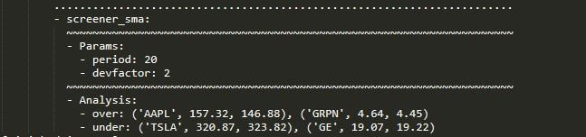
We tin see that TSLA and GE traded at least two standard deviations beneath their average shut cost over the prior 20 days on October 30, 2017.
How to lawmaking an indicator in Backtrader
At that place are three ways to code an indicator in Backtrader. You can code one from scratch, utilize a built-in indicator, or use a third-political party library.
If you don't program to use the live trading functionality of Backtrader, yous might want to code your indicator yourself.
Here is an instance of an indicator we created:
range_total = 0 for i in range(-13, ane): true_range = self.datahigh[i] - cocky.datalow[i] range_total += true_range ATR = range_total / 14
The above code calculates the Average True Range (ATR). Its aim is to requite an estimate of how much an instrument will typically fluctuate in a given period.
It does this by iterating through the concluding 14 data points which can be done in Backtrader past using a negative index. We take the high and decrease the low for each period, and then average information technology out.
The code can then exist placed inside the next function of our strategy class. We can too add a simple log part to log the indicator to the screen like this:
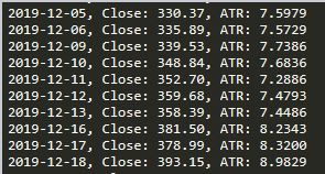
cocky.log(f'Close: {cocky.dataclose[0]:.2f} ATR: {ATR:.4f}') Here is the complete strategy code:
course AverageTrueRange(bt.Strategy): def log(self, txt, dt=None): dt = dt or self.datas[0].datetime.engagement(0) print(f'{dt.isoformat()} {txt}') #Print appointment and close def __init__(self): self.dataclose = self.datas[0].close self.datahigh = cocky.datas[0].high cocky.datalow = cocky.datas[0].low def adjacent(self): range_total = 0 for i in range(-13, ane): true_range = self.datahigh[i] - cocky.datalow[i] range_total += true_range ATR = range_total / xiv self.log(f'Close: {self.dataclose[0]:.2f}, ATR: {ATR:.4f}') Here is what the output looks like when nosotros put information technology all together.
Yous can check out ChartSchool to learn the mathematics and code behind different technical indicators.
How to plot in Backtrader
To plot a chart in Backtrader is incredibly simple. All yous need to do is add cerebro.plot() to your code after calling cerebro.run().
Here is an example of a chart with the TSLA data nosotros've been using in our examples.
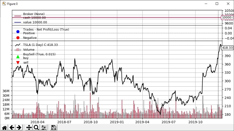
By default, the nautical chart will endeavor to show the post-obit
- Fluctuations in your balance
- The profit or loss of any trades taken during the backtest
- Where buy and sell trades took place relative to the price.
If you're not interested in seeing all of these boosted details, merely laissez passer through the following parameter – stdstats=False. Y'all tin pass information technology through either when you instantiate cerebro, or when you call cerebro.run. Both will produce the aforementioned result.
Retrieve that we used this parameter in our stock screener?
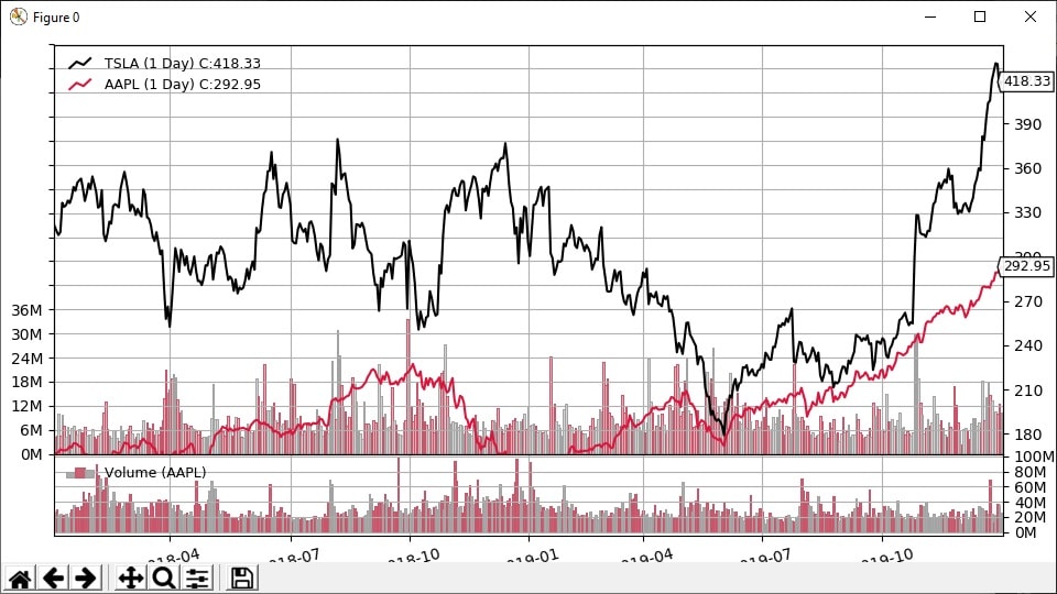
If you're working with ii different stocks, you can hands bear witness both on one chart. This can be useful if you lot're trying to visualize the correlation betwixt 2 assets.
import datetime import backtrader as bt #Instantiate Cerebro engine cerebro = bt.Cerebro(stdstats=Simulated) #Ready data parameters and add to Cerebro data1 = bt.feeds.YahooFinanceCSVData( dataname='TSLA.csv', fromdate=datetime.datetime(2018, ane, ane), todate=datetime.datetime(2020, i, 1)) cerebro.adddata(data1) data2 = bt.feeds.YahooFinanceCSVData( dataname='AAPL.csv', fromdate=datetime.datetime(2018, i, 1), todate=datetime.datetime(2020, 1, i)) data2.recoup(data1) # let the system know ops on data1 affect data0 data2.plotinfo.plotmaster = data1 data2.plotinfo.sameaxis = True cerebro.adddata(data2) #Run Cerebro Engine cerebro.run() cerebro.plot() The above lawmaking volition create a nautical chart with TSLA and AAPL price information overlaid on summit of each other. This is what the nautical chart looks similar:

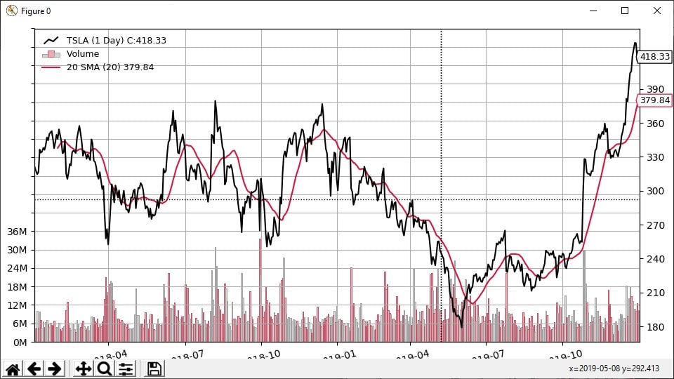
Lastly, any indicator you lot might add volition automatically get added to the chart. Here is a code instance that will bear witness TSLA toll data with a 20-twenty-four hour period moving average.
import datetime import backtrader as bt #simple moving average class SimpleMA(bt.Strategy): def __init__(self): self.sma = bt.indicators.SimpleMovingAverage(self.data, menstruation=twenty, plotname="20 SMA") #Instantiate Cerebro engine cerebro = bt.Cerebro(stdstats=False) #Prepare data parameters and add to Cerebro data1 = bt.feeds.YahooFinanceCSVData( dataname='TSLA.csv', fromdate=datetime.datetime(2018, ane, 1), todate=datetime.datetime(2020, one, 1)) cerebro.adddata(data1) cerebro.addstrategy(SimpleMA) #Run Cerebro Engine cerebro.run() cerebro.plot() Observe nosotros passed through a value for plotname. It allows the states to change the display value for the moving average in the legend. This is what the nautical chart looks like:
How to use culling data in Backtrader
In this strategy, we're going to try and judge sentiment based on google search information, and execute trades based on any notable shifts in search volume.
We've downloaded historical weekly search information from Google Trends for Bitcoin and have obtained cost information from Yahoo Finance.
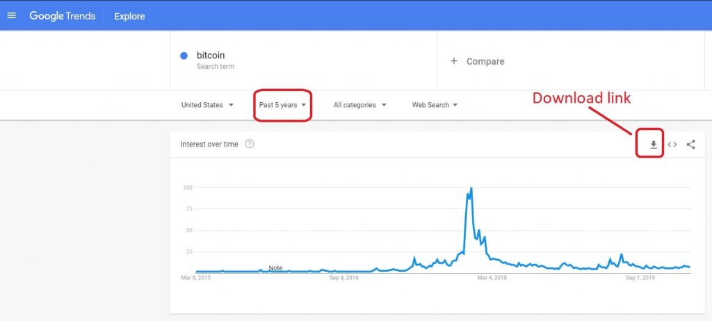
Since in that location was a lot of volatility in late 2017, we will test this strategy from 2018 onward. Search results information and prices both stabilized quite a bit after that betoken.
The Google Trends data we've downloaded does not follow the same open, high, low, close format as our Yahoo Finance information. Therefore, we will apply the generic CSV template provided by Backtrader to add in our data. Hither is the code:
data2 = bt.feeds.GenericCSVData( dataname='BTC_Gtrends.csv', fromdate=datetime.datetime(2018, 1, i), todate=datetime.datetime(2020, one, ane), nullvalue=0.0, dtformat=('%Y-%k-%d'), datetime=0, time=-ane, high=-ane, low=-1, open=-1, close=ane, volume=-1, openinterest=-1, timeframe=bt.TimeFrame.Weeks) cerebro.adddata(data2) We had to define which columns were present and which weren't. This was done by assigning -1 values for columns non nowadays in our data and assigning an incrementing integer value for columns that were available.
Aside from that, our main code script was pretty much unchanged from the moving average crossover example.
Here is our strategy course:
form BtcSentiment(bt.Strategy): params = (('period', 10), ('devfactor', i),) def log(self, txt, dt=None): dt = dt or self.datas[0].datetime.appointment(0) print(f'{dt.isoformat()} {txt}') def __init__(self): self.btc_price = self.datas[0].close cocky.google_sentiment = self.datas[one].close cocky.bbands = bt.indicators.BollingerBands(self.google_sentiment, catamenia=self.params.period, devfactor=self.params.devfactor) self.order = None def notify_order(self, lodge): if guild.status in [order.Submitted, order.Accustomed]: # Existing guild - Nothing to do render # Check if an order has been completed # Attention: broker could reject society if non plenty cash if order.status in [order.Completed]: if social club.status in [order.Completed]: if order.isbuy(): cocky.log(f'Buy EXECUTED, {order.executed.price:.2f}') elif order.issell(): self.log(f'SELL EXECUTED, {order.executed.toll:.2f}') self.bar_executed = len(self) elif social club.status in [order.Canceled, order.Margin, guild.Rejected]: self.log('Society Canceled/Margin/Rejected') # Reset orders self.society = None def next(cocky): # Cheque for open up orders if self.order: render #Long signal if self.google_sentiment > cocky.bbands.lines.superlative[0]: # Check if we are in the market if not self.position: self.log(f'Google Sentiment Value: {self.google_sentiment[0]:.2f}') self.log(f'Top band: {self.bbands.lines.elevation[0]:.2f}') # We are not in the market place, we volition open a trade self.log(f'***Buy CREATE {self.btc_price[0]:.2f}') # Keep track of the created order to avoid a 2nd order self.order = self.buy() #Short bespeak elif self.google_sentiment < cocky.bbands.lines.bot[0]: # Bank check if nosotros are in the market if not self.position: self.log(f'Google Sentiment Value: {self.google_sentiment[0]:.2f}') self.log(f'Bottom band: {self.bbands.lines.bot[0]:.2f}') # We are not in the marketplace, we will open up a trade self.log(f'***SELL CREATE {self.btc_price[0]:.2f}') # Continue track of the created order to avert a 2nd society self.guild = cocky.sell() #Neutral bespeak - close any open trades else: if self.position: # We are in the market, we volition close the existing trade cocky.log(f'Google Sentiment Value: {self.google_sentiment[0]:.2f}') self.log(f'Bottom band: {self.bbands.lines.bot[0]:.2f}') cocky.log(f'Summit band: {cocky.bbands.lines.top[0]:.2f}') self.log(f'CLOSE CREATE {self.btc_price[0]:.2f}') self.guild = cocky.close() Nosotros are once once again using Bollinger bands. The above script looks for a rise greater than one standard deviation in search volume to enter a long position and vice versa to enter short.
If the search information retreats dorsum inside one standard deviation of the average of the last 10 data points, we volition shut our position.
In the __init__ function, we assigned variable names to the two different datasets so that we tin can reference them easier throughout our strategy. Bated from this, the syntax is very similar to the prior examples.
After running the backtest, hither are our results:
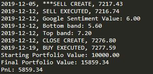
The strategy made a whopping $5859 on a $10,000 starting balance. That's a most threescore% render! And that's without trying to run any optimization.
How to add visual stats to a backtest
Backtrader has quite a few analyzers that provide in-depth detail of the backtest. Merely rather than programming several analyzers, we tin employ a third-party library which will prove complete statistics of the backtest too equally other visualizations.
A pop library for this is PyFolio which can create a detailed tearsheet with all sorts of information. This is done via Jupyter notebooks.
Another good option is to utilize the quantstats library. The do good of this library is that it saves an HTML file of the stats, eliminating the additional step of running a notebook that PyFolio requires.
The easiest fashion to install quantstats is by pip through the command line.
pip install quantstats Both quantstats and PyFolio require returns data to calculate stats. We can utilise a Backtrader analyzer to get this information.
We will build on our previous culling information example and create a stats tearsheet from our BTC sentiment strategy. The first footstep is to add the analyzer that volition requite the states returns data. Nosotros need to add the following line of code:
cerebro.addanalyzer(bt.analyzers.PyFolio, _name='PyFolio') The above line of code can be added anywhere in the script as long as information technology'south earlier the cerebro.run command and after initializing the cerebro class.
Every bit you may have guessed from the proper noun, this analyzer was created to enable a PyFolio integration. But it works just also with the quantstats library.
We volition need to save the results from our backtest, like to what nosotros did in the Sharpe Ratio example.
results = cerebro.run() strat = results[0] At the end of our script, later on our backtest completes, nosotros can add some code to extract the returns data from the analyzer.
portfolio_stats = strat.analyzers.getbyname('PyFolio') returns, positions, transactions, gross_lev = portfolio_stats.get_pf_items() returns.alphabetize = returns.index.tz_convert(None) The above lawmaking gets all the information obtained by the PyFolio analyzer. We then dissever the returned information to extract just the returns values.
As you may have guessed from the proper noun, this analyzer was created to enThe returns variable is actually a Pandas DataFrame. To get in uniform with quantstats, we removed the timezone awareness using the built-in tz_convertfunction from Pandas.
Since we are using Pandas, nosotros have to import it into our script. We tin also import the quantstat library at the aforementioned fourth dimension. We'll add together the post-obit at the summit of our script to do that.
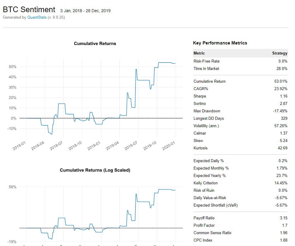
import pandas equally pd import quantstats Let's jump back to the lesser of the script and add the functionality to create a stats tearsheet.
quantstats.reports.html(returns, output='stats.html', title='BTC Sentiment') After running the backtest again, a stats.html file is created in our projects folder. It looks like this:
How to relieve backtest information to a CSV file
In the examples here, we've printed opened and closed trades to the console. Merely if you're running multiple tests and later on want to compare them, it might be useful writing your backtest data to a CSV file.
There is a born method in backtrader that will create a CSV file for you. It includes data from your information feeds, strategies, indicators, and analyzers.
To utilize it, simply add the following line to your script. It can be added anywhere in the script equally long as it is before cerebro.run and after instantiating the cerebro class.
cerebro.addwriter(bt.WriterFile, csv=Truthful, out='log.csv') For theoutparameter, we've specifiedlog.csv. You can proper name the file anything y'all want. After running your backtest, there should be a CSV file in your projects directory with all of the earlier mentioned data.
At that place are other options also if you'd like a more than customized arroyo. Within the strategy course, nosotros can overwrite the cease() function to save whatever variable within the form. Here is an case.
class BtcSentiment(bt.Strategy): def __init__(cocky, sp): cocky.log_pnl = [] In the __init__ office, we've initialized a variable chosen log_pnl as a list.
def log(cocky, txt, dt=None): dt = dt or self.datas[0].datetime.date(0) print(f'{dt.isoformat()} {txt}') #Impress date and close self.log_pnl.append(f'{dt.isoformat()} {txt}') Then under the log function, we're appending the output (what would normally be printed to the console) to our log_pnl list.
Finally, we can save the list to a file once the backtest is finished running. For this, nosotros use the cease() part which runs one time when the backtest is complete. Here is the code to save the log_pnl to file.
def finish(self): with open('custom_log.csv', 'westward') as eastward: for line in self.log_file: e.write(line + '\n') You can use this method to save any custom data from backtrader to a file.
In our previous example, nosotros used the backtrader PyFolio analyzer to generate returns and other data that took the form of a Pandas DataFrame. We tin relieve the returns data, or whatsoever of the other files past using the built-in to_csv() method from Pandas.
returns.to_csv('returns.csv')) Alternatives to Backtrader
At that place are a lot of choices when it comes to backtesting software although in that location were 3 names that popped up often in our enquiry – Zipline, PyAlgoTrade, and Backtrader.
Interestingly, the author of Backtrader decided on creating it afterward playing around with PyAlgoTrade and finding that it lacked the functionality that he was seeking.
And information technology looks like he'due south test-driven a few other backtesting platforms equally well. If you're looking for a larger list of alternatives, cheque out the Backtrader GitHub page which has a list of 20 alternatives.
Last Thoughts on Backtrader
It is clear a lot of piece of work has gone into Backtrader and it delivers more than than what the average user is likely looking for. This could have easily become a commercial solution and nosotros commend the author for keeping it open-source.
Subsequently going through this tutorial, you should be in a good position to endeavour out your get-go strategy in Backtrader. There are a few additional points that we suggest you lot look into and endeavour to incorporate into your backtesting.
Commissions – Trading fees and commissions add up and these should not exist ignored. Backtrader initially only allowed users to set a percentage-based commission for stocks but this has since evolved to adjust fixed pricing.
Risk Management – our examples did non incorporate much in terms of risk direction. The objective here was to highlight the potential of Backtrader and provide a solid foundation for using the platform.
Your backtesting results will probable vary a great deal depending on what type of risk management you lot implement. The goal is to optimize your strategy to all-time align with your risk tolerance rather than attempting to maximize profits at the cost of taking nifty risks.
Lastly, the focus when it comes to strategy development should exist to come up with a good foundation and then use optimization for minor tweaks. Sometimes traders fall into the trap of approaching it the other way around which rarely leads to a profitable strategy.
Download code
Github link
Source: https://algotrading101.com/learn/backtrader-for-backtesting/
Enviar um comentário for "Quantopian How to Use Custom Uploaded Data"